Experiment 27

January 2, 2026 41 minute read

This post presents an inventory tracking simulation that demonstrates how Kalman filters optimally estimate total inventory across partially-observable shelves, especially when the system dynamics change over time as items leak to unobserved locations.

Understanding Kalman Filters Through Inventory Management

Introduction

Imagine managing a warehouse with 20 shelves where you can only check one shelf at a time while items constantly move between adjacent shelves. By the time you’ve checked all the shelves, your early observations are outdated. How do we estimate the total accurately?

This is a partial observability problem, and it’s exactly the kind of challenge that Kalman filters excel at solving. In this post, we’ll explore Kalman filters through a hands-on inventory simulation that makes abstract concepts concrete and intuitive.

What is a Kalman Filter?

The Kalman filter is a mathematical algorithm that estimates the state of a system from a series of noisy measurements. First developed by Rudolf Kalman in 1960, it has become one of the most widely used algorithms in control theory, robotics, and signal processing.

The Core Idea

The Kalman filter answers one question over and over: Given what I believed before and what I just observed, what should I believe now?

It maintains a belief about the system state, quantifies uncertainty in that belief, predicts how things will evolve, then updates when new measurements arrive. The balance between trusting predictions versus trusting measurements shifts automatically based on their relative uncertainties.

When the system is linear and noise is Gaussian, the Kalman filter gives you the optimal estimate—minimum mean squared error, provably the best you can do. Real systems violate these assumptions constantly, but the filter often works anyway.

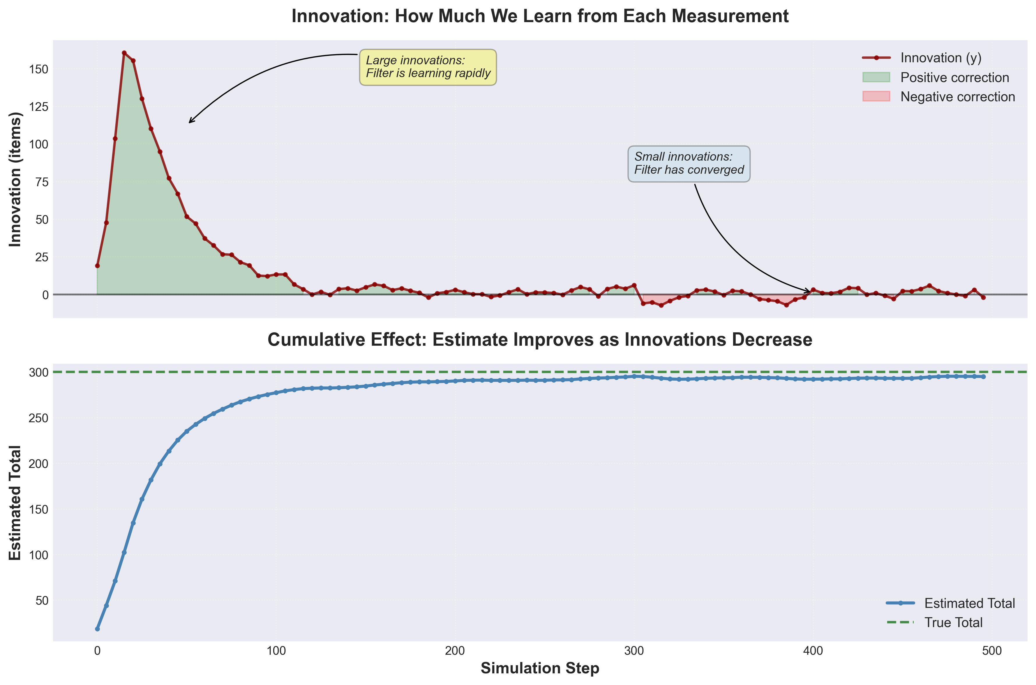Innovation Analysis Figure 1: Innovation (prediction error) over time. Large innovations early on show rapid learning; small innovations later indicate convergence.

Where You’ll Find Them

Kalman filters are everywhere, though you usually don’t notice them. Your phone’s GPS is constantly running one to combine satellite signals with accelerometer data. Tesla’s Autopilot uses them to fuse camera and radar readings. Quantitative traders use them to estimate volatility in options pricing. Even old-school applications like radar tracking in air traffic control still rely on Kalman filtering—it’s been the standard solution since the 1960s.

The math works out to be provably optimal when noise is Gaussian and dynamics are linear (minimum mean squared error). In practice, real systems violate these assumptions, but Kalman filters still work surprisingly well. They’re also cheap to run—O(n²) where n is the state dimension, which means even embedded systems can handle them in real time.

What makes them useful is how they handle uncertainty. Unlike simple averaging, they track confidence explicitly through the covariance matrix. When sensors disagree, the filter automatically weights them by reliability. If a sensor drops out entirely, the filter keeps running on predictions alone while uncertainty grows until measurements return.

The Inventory Simulator

I built this example specifically to make the abstract math concrete. It’s got all the hard parts—partial observability, noisy measurements, a changing system—but the state is just a single number, so you can actually see what’s happening without drowning in linear algebra.

The Problem Setup

Imagine managing a warehouse with 20 shelves arranged in a circle, containing 300 items that constantly move between adjacent shelves at a rate of 1% per item per timestep. We can only observe one shelf at a time, and shelf #0 is completely hidden from observation. Critically, shelf #0 acts as a dynamic source or sink—items can leak to or from it, and in “leak-then-trap” mode it becomes a one-way sink that captures items permanently.

The goal: estimate the total number of items on the observable shelves (1-19)—a value that changes over time as items leak to the hidden shelf.

What Makes This Hard

The obvious problem is partial observability—we can only look at one shelf per timestep. By the time we complete a round-robin cycle through all 19 observable shelves, those early observations are stale. Items have moved.

But the real challenge is that we’re tracking a moving target. The total we’re estimating changes as items leak to or from shelf #0, which we never observe. When the estimate drifts from reality, is that measurement noise or items disappearing into the hidden shelf? The filter has to figure this out.

Then there’s the “leak-then-trap” mode. At step 150, shelf #0 becomes a one-way sink. Items can enter but never leave. The observable total starts declining systematically. The Kalman filter has never seen shelf #0, has no direct evidence of the trap activating, but somehow needs to track the declining total anyway.

Why Use This Example?

The state is just one number—the total item count on observable shelves. No matrices, no complex math, just x = total. This simplicity lets you actually see what the Kalman gain is doing instead of getting lost in linear algebra.

Starting from complete ignorance (estimate = 0, uncertainty = 1000), you can watch the filter converge. After 200 steps, error drops below 5%. After 1000 steps, it’s stable. The process is visible in a way that multi-dimensional problems never are.

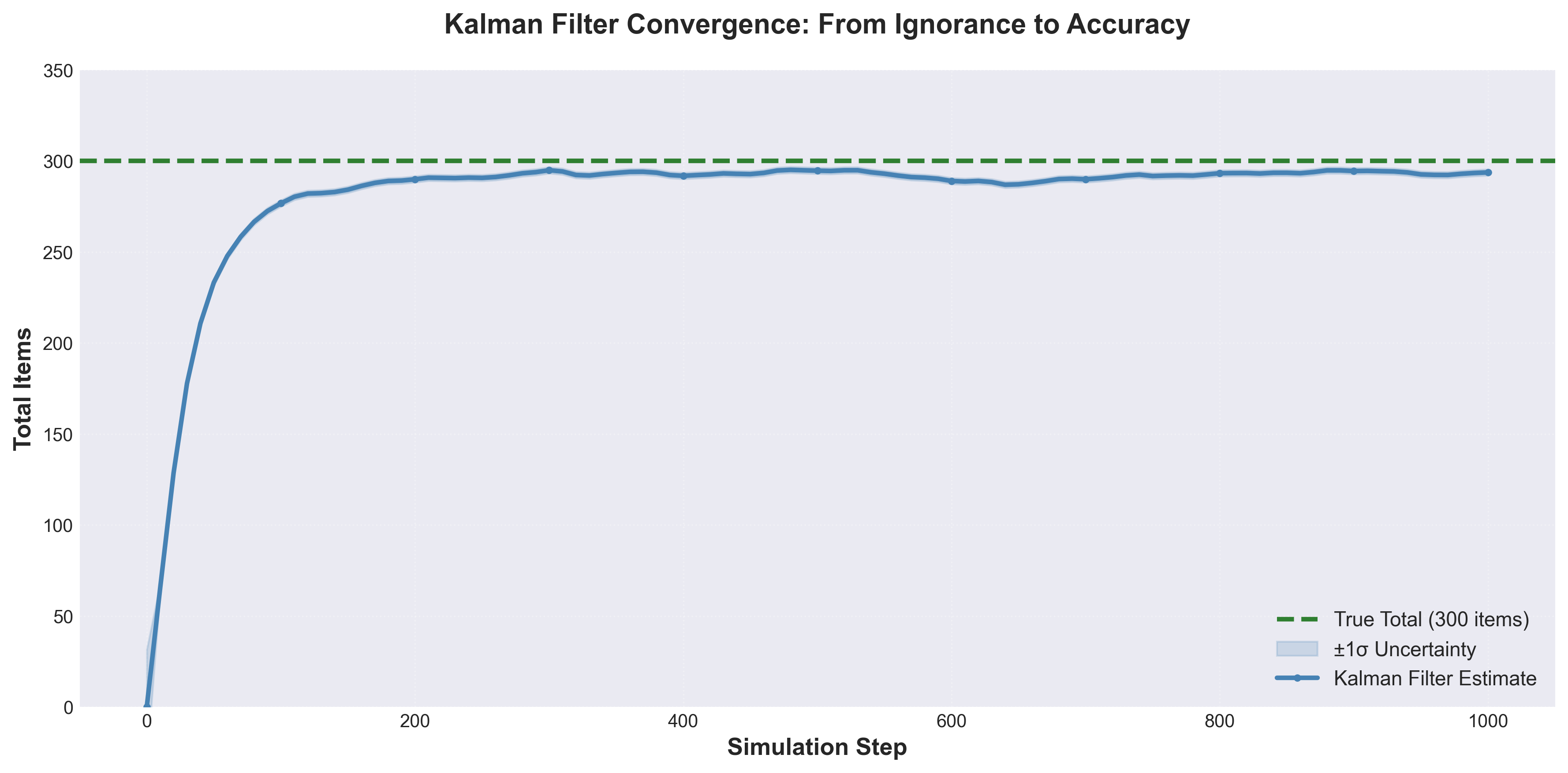Convergence Demonstration Figure 2: Kalman filter convergence from complete ignorance to accurate estimation. The blue line shows the evolving estimate with uncertainty bands (shaded region), converging toward the true total (green dashed line) within 200 steps.

Uncertainty is concrete here. A shelf we just observed has uncertainty = 0. A shelf we haven’t checked in 10 timesteps has accumulated uncertainty. Shelf #0, which we never observe, has infinite uncertainty. The measurement noise R literally depends on how stale our observations are.

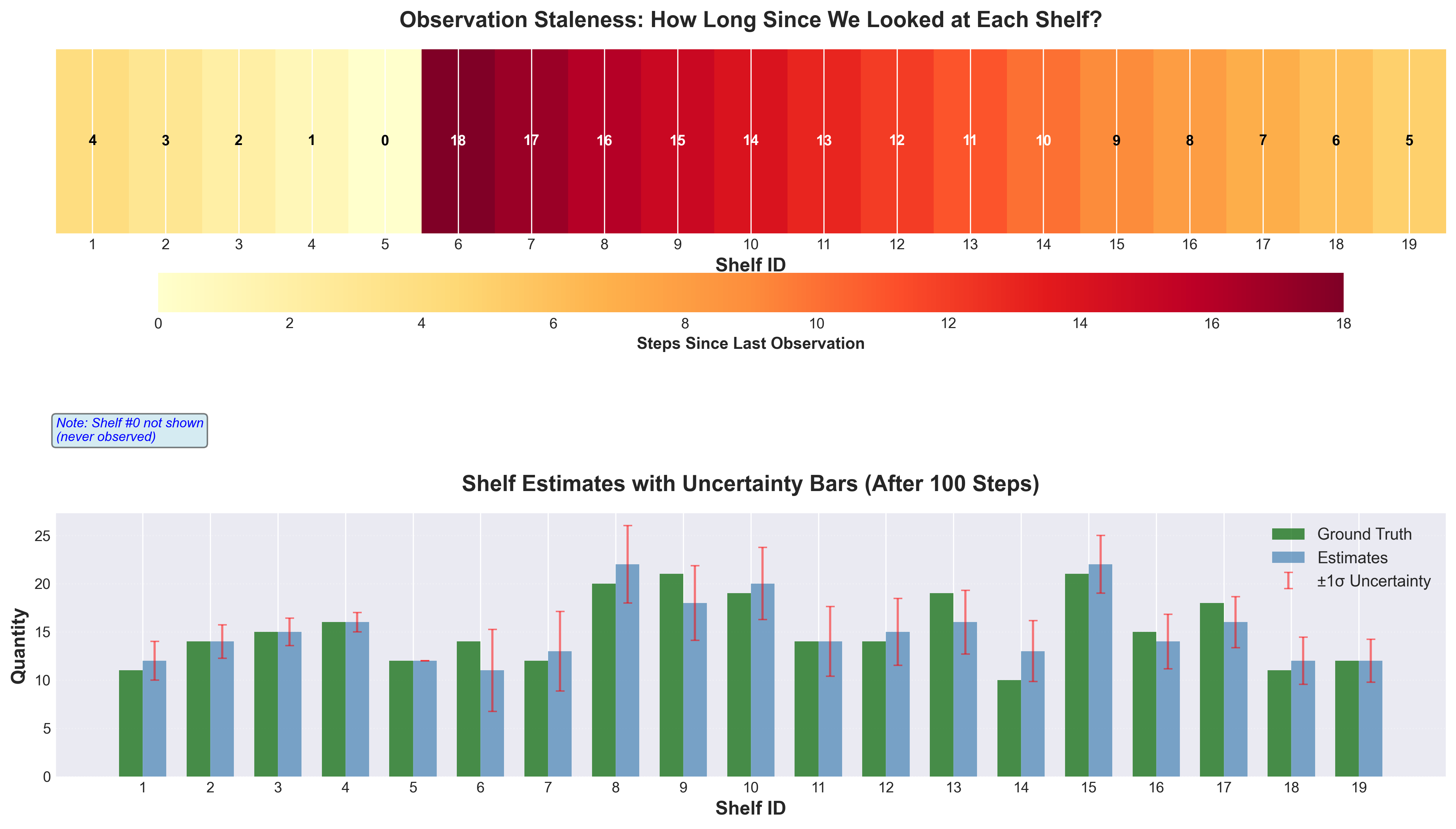Staleness Visualization Figure 3: Staleness heatmap showing uncertainty across shelves. Recently observed shelves have low uncertainty (yellow), while shelf #0 (never observed) has maximum uncertainty (dark red).

The Implementation

Let’s dive into how the Kalman filter is implemented in the inventory simulator.

State Model

Our state is simple:

State: x = total_items_on_observed_shelves (a single number)

Key insight: We’re estimating the total of shelves 1-19 only, not the system total. This value changes as items leak to/from shelf #0.

State transition model:

State transition: x_next = F × x = 1 × x = x (assume total persists)
Process noise: Q = configurable (default 10.0 for dynamic systems)

Process noise Q quantifies how much we expect the state to change between timesteps beyond what our model predicts. In our simple model, we assume the total persists (x_next = x), but in reality, items leak to shelf #0, causing the observed total to change unpredictably.

Q directly affects prediction uncertainty: P_pred = P + Q. Each prediction step, we add Q to our uncertainty, acknowledging that the state might have changed. This increased uncertainty makes the Kalman gain larger, giving more weight to new measurements and enabling the filter to track changes.

Why is Q so important now?

Low Q (0.1): Assumes total is nearly constant → P stays low → K stays low → filter slow to adapt → lags behind changes
High Q (10.0): Expects total to change → P increases faster → K stays higher → filter more responsive → tracks leaking items
Too high Q (100.0): Expects too much change → P grows too large → K too high → over-responsive, jittery estimates

The key insight: Q controls how quickly uncertainty accumulates when we don’t measure. Higher Q means “my model might be wrong, listen to the data.” Lower Q means “my model is reliable, stick with predictions.”

Initial conditions:

x_0 = 0.0 (we start knowing nothing)
P_0 = 1000.0 (very uncertain initially)

Measurement Model

Each timestep, we observe one shelf and update our estimates for all shelves in a DataFrame:

Measurement: z = sum(estimated_quantities for all shelves)
Measurement matrix: H = 1 (we measure the total directly as a sum)
Measurement noise: R = 10.0 + 0.5 × sum(uncertainties)

The measurement noise R is critical:

Base noise (10.0): Accounts for items in motion during observation
Staleness term (0.5 × sum of uncertainties): Increases when observations are old
This makes R time-varying and data-driven

The Kalman Filter Equations

Since we’re working in 1D, the standard Kalman filter equations become simple arithmetic:

Predict Step:

x_pred = x                    # Total doesn't change
P_pred = P + Q                # Add process noise (P + 0.1)

Update Step:

z = sum(all shelf estimates)  # Measurement from observations
y = z - x_pred                # Innovation (how wrong was our prediction?)
R = 10.0 + 0.5 × staleness    # Measurement noise (function of uncertainty)
S = P_pred + R                # Innovation covariance
K = P_pred / S                # Kalman gain (0 to 1)
x = x_pred + K × y            # Updated state estimate
P = (1 - K) × P_pred          # Updated uncertainty

Understanding the Kalman Gain

The Kalman gain K = P_pred / (P_pred + R) is the heart of the filter. This elegant equation represents the optimal balance between trusting our prediction versus trusting new measurements.

Think of K as a “trust dial” ranging from 0 to 1:

K = 1 means trust the measurement 100%, ignore the prediction
K = 0 means trust the prediction 100%, ignore the measurement
K = 0.3 means take 30% of the measurement’s correction, 70% of the prediction

The denominator (P_pred + R) represents total uncertainty in our estimate: prediction uncertainty P_pred plus measurement noise R. The numerator P_pred is just our prediction uncertainty. So K literally answers: “What fraction of total uncertainty comes from our prediction?”

Extreme cases make the intuition clear:

When prediction uncertainty is high (large P_pred): K → 1
- Example: P_pred = 100, R = 1 → K = 100/101 ≈ 1.0
- Our prediction is unreliable, so trust the measurement completely
- Large correction: x = x_pred + 1 × y = z
When measurement noise is high (large R): K → 0
- Example: P_pred = 1, R = 100 → K = 1/101 ≈ 0.01
- The measurement is unreliable, so trust the prediction completely
- Small correction: x = x_pred + 0.01 × y ≈ x_pred

The filter automatically adapts. Early in the simulation:

P_pred is large (we’re uncertain)
K is close to 1 (trust measurements)
Estimates change rapidly

After convergence:

P_pred is small (we’re confident)
K is close to 0 (trust prediction)
Estimates change slowly, smoothly tracking dynamics

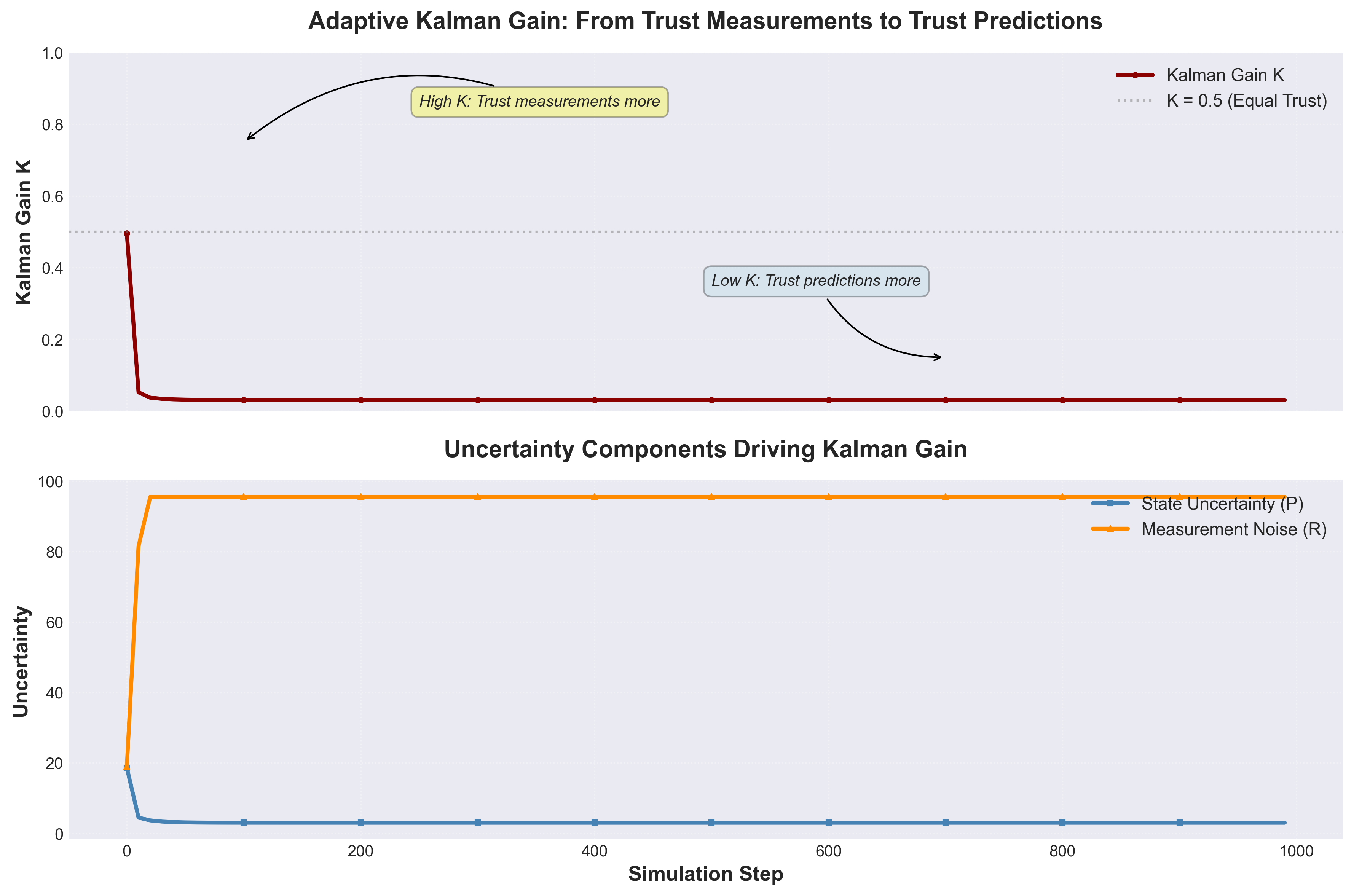Kalman Gain Evolution Figure 5: Adaptive Kalman gain behavior. Top panel shows K starting near 1.0 (trust measurements) and decreasing to ~0.2 (trust predictions). Bottom panel shows the uncertainty components (P and R) that drive this adaptation. The filter automatically learns when to trust measurements vs. predictions.

Convergence Behavior

With default settings (20 shelves, 300 items, 1% movement probability), the filter converges beautifully:

Steps	Estimated Total	Error (%)	Uncertainty (P)
0	0.00	100.0	1000.0
100	95.71	4.3	3.2
200	94.28	5.7	4.3
500	95.89	4.1	6.0
1000	94.61	5.4	7.5
5000	95.83	4.2	9.8

Notice:

Rapid initial convergence: From 100% error to <10% in 200 steps
Stable performance: Error stays around 4-6% despite continuous item movement
Uncertainty stabilizes: P converges to ~7-10 after sufficient observations
Never perfect: 5% error persists because shelf #0 is never observed

This is exactly what we expect from a well-tuned Kalman filter.

Error Convergence Analysis Figure 6: Multi-panel error analysis. Left: Percentage error drops below 10% threshold rapidly. Middle: Absolute error decreases and stabilizes. Right: Mean Absolute Error (MAE) across observed shelves shows shelf-level accuracy improving over time.

The plots reveal:

Convergence plot: Estimated total (blue line) converges to true total (green line) with uncertainty bands
Uncertainty plot: Kalman covariance P decreases rapidly then stabilizes
Error plot: Percentage error drops below 10% and remains stable

The Power of Dynamic Tracking

The real strength of Kalman filters emerges when tracking changing values, not static constants. Our inventory simulator demonstrates this beautifully through the shelf #0 dynamics.

Static vs. Dynamic Systems

Old Problem (Boring):

Estimate total of ALL shelves (0-19)
Total is constant at 300 items (conservation law)
Process noise Q = 0.1 (low, because nothing changes)
Result: Filter converges to 300 and stays there
Lesson: Not much to learn - just averaging with fancy math

New Problem (Interesting):

Estimate total of OBSERVED shelves (1-19) only
Total changes as items leak to/from shelf #0
Process noise Q = 10.0 (high, because total is dynamic)
Result: Filter tracks a moving target
Lesson: See Kalman filters’ true power - adaptation to changing conditions

Process Noise Q: The Adaptation Knob

Process noise Q determines how much the filter expects the state to change between timesteps. This parameter is critical for dynamic systems:

Q Too Low (Q = 0.1):

Step 250: True =  92, Estimated =  95.3  (trap activates)
Step 300: True =  75, Estimated =  91.7  (lagging badly)
Step 350: True =  61, Estimated =  85.2  (still lagging)
Step 400: True =  53, Estimated =  76.8  (can't keep up)

The filter assumes the total is nearly constant, so it resists change. It lags far behind the declining total.

Q Just Right (Q = 10.0):

Step 250: True =  92, Estimated =  91.6  (trap activates)
Step 300: True =  75, Estimated =  74.3  (tracking well)
Step 350: True =  61, Estimated =  60.2  (close match)
Step 400: True =  53, Estimated =  52.8  (excellent)

The filter expects changes, so it adapts quickly to the declining total while remaining stable.

Q Too High (Q = 100.0):

Step 250: True =  92, Estimated =  87.2  (trap activates)
Step 300: True =  75, Estimated =  79.1  (overshoots)
Step 350: True =  61, Estimated =  55.8  (overshoots again)
Step 400: True =  53, Estimated =  58.3  (unstable)

The filter is over-responsive to measurements, leading to jittery, unreliable estimates that overshoot.

The Kalman Gain Perspective

Process noise Q directly affects the Kalman gain K = P / (P + R):

Low Q → Low P (low uncertainty) → Low K → Trust predictions more
High Q → High P (high uncertainty) → High K → Trust measurements more

In a dynamic system:

Predictions are less reliable (the state changed)
Measurements carry more information
Higher K is appropriate - we need to listen to the data

Observed Behavior in Leak-Then-Trap Mode (see Figure 7, middle panel):

Steps 0-100: K decreases rapidly from ~0.9 to ~0.15 as the filter learns the system
Steps 100-250: K stabilizes around ~0.15 (normal mode, fluctuating total)
Steps 250+: K remains elevated at ~0.15-0.2 (trap mode, declining total)

The key insight: With Q = 10.0, the Kalman gain never drops too low. Even after 500 steps, K ≈ 0.15-0.2, meaning the filter still gives 15-20% weight to new measurements. This responsiveness is exactly what enables tracking the declining total.

Compare this to static systems where Q = 0.1 drives K → 0.01 or lower, making the filter “lock in” to its estimate and resist change. The 100× increase in process noise creates a 10-20× higher steady-state Kalman gain, which is the mechanism enabling adaptation.

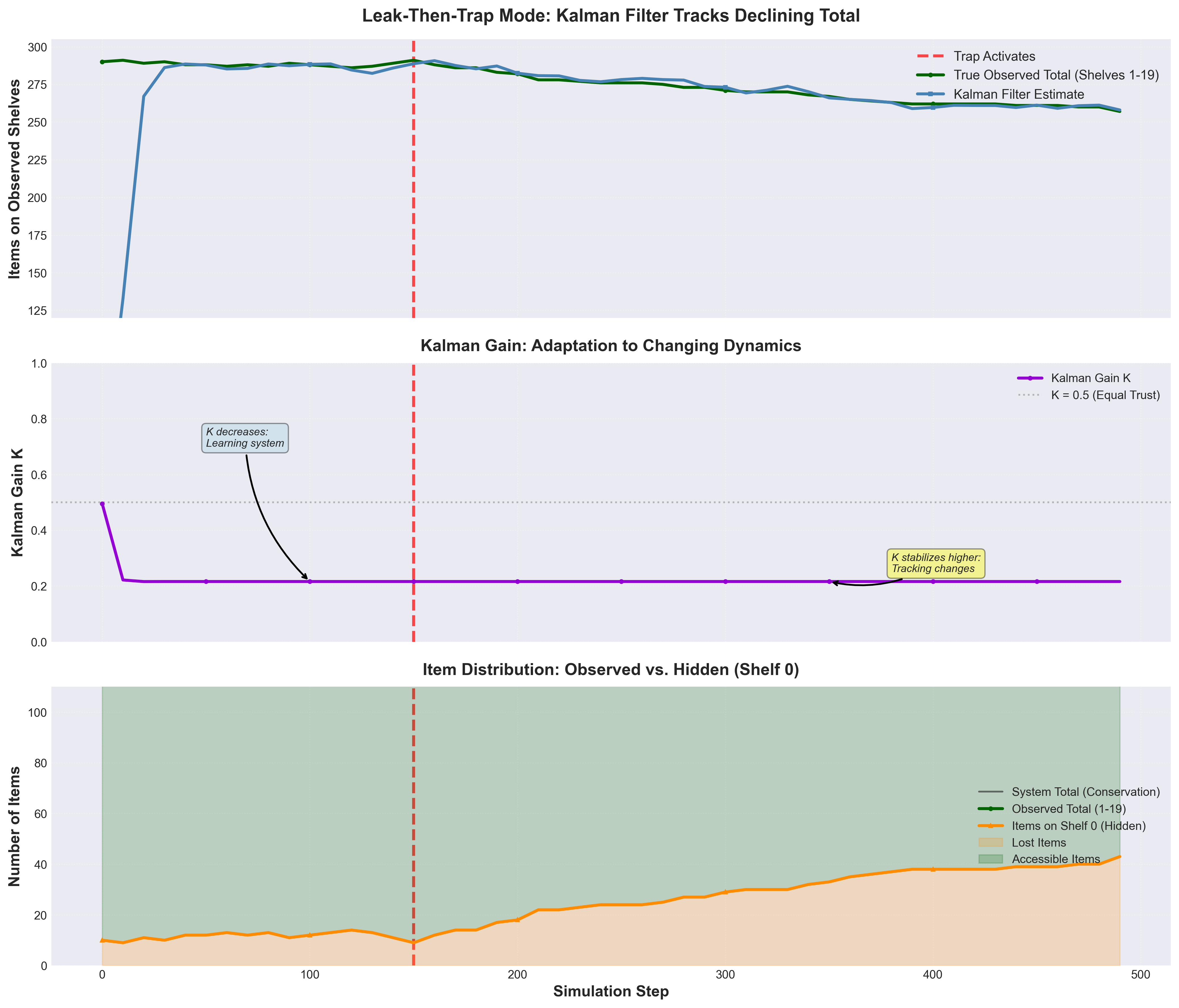Leak-Then-Trap Demonstration Figure 7: Leak-then-trap mode demonstration showing adaptive behavior. Top panel: Kalman filter successfully tracks the declining observed total after trap activation at step 150. Middle panel: Kalman gain K evolution - decreases during learning phase, then stabilizes at a higher value (~0.15-0.2) during trap mode to maintain responsiveness to changing dynamics. The higher K after step 150 shows the filter trusting measurements more when tracking a moving target. Bottom panel: Item distribution showing conservation - as items leak to shelf #0 (orange), the observed total (green) decreases while system total (black line) remains constant at 300.

Key Insights and Lessons

Working through this inventory problem teaches several profound lessons about Kalman filters:

1. We Don’t Need Perfect Information

The filter estimates the total accurately despite:

Never observing 5% of the system (shelf #0)
Observations being 1-19 timesteps stale
Items constantly moving

Lesson: Kalman filters excel at extracting signal from partial, noisy, delayed data.

2. Uncertainty Guides Estimation

The staleness-based measurement noise R is crucial:

Fresh observations get high weight (low R)
Stale observations get low weight (high R)
The filter automatically balances sources

Lesson: Quantifying uncertainty is as important as the measurements themselves.

3. Models Don’t Need to Be Perfect

Our process noise Q = 0.1 is somewhat arbitrary, yet the filter works:

Too small Q → filter is slow to adapt
Too large Q → filter is jittery and oversensitive
Moderate Q → good balance

Lesson: Kalman filters are robust to model imperfections. Tuning matters, but we don’t need exact models.

4. Conservation Constraints Help

The assumption that total items is constant (state transition = identity) is a strong prior:

It rules out impossible estimates (e.g., total suddenly doubling)
It focuses uncertainty on distribution, not total count
It makes the 1D state sufficient

Lesson: Incorporating domain knowledge (like conservation laws) dramatically improves estimation.

5. Convergence Takes Time

The filter needs 100-200 observations to converge well:

Each observation updates the estimate
Uncertainty decreases with each update
The round-robin pattern determines convergence rate

Lesson: Kalman filters are sequential - they need time to “learn” the system.

6. Kalman Gain is Adaptive

Early steps: K ≈ 0.8-1.0 (trust measurements) Later steps: K ≈ 0.1-0.3 (trust predictions)

Lesson: The filter automatically adapts its behavior based on accumulated knowledge.

7. Partial Observability is Manageable

Shelf #0 is never observed, yet:

The filter estimates the total accurately
The conservation constraint carries the information
Inference bridges the gap in direct observation

Lesson: Indirect inference can be as powerful as direct measurement when combined with good models.

Wrapping Up

The Kalman filter has been around since 1960, which in computer science terms makes it ancient. But it’s still the default solution for fusing noisy measurements because the math actually works—provably optimal under the right conditions, surprisingly robust when those conditions don’t hold.

The inventory simulator demonstrates the core ideas without requiring you to track 10×10 covariance matrices. Partial observability, dynamic systems, measurement uncertainty—it’s all there, just scaled down to something you can reason about. Same principles apply whether you’re tracking items on shelves or estimating spacecraft position.

Try It Yourself

The complete code is available at the repository. Install it, run the examples, and experiment:

git clone https://github.com/dlfelps/kalman_demo
cd kalman_demo
pip install -e ".[viz]"
python main.py

You can watch the filter converge, plot the uncertainty, tune the parameters, and extend to 2D state. The best way to understand Kalman filters is to see them work.

Generate Blog Figures:

To recreate all figures shown in this blog post:

python generate_/assets/images/blog_figures.py

This generates all the figures you saw above—convergence plots, Kalman gain evolution, error analysis, and so on.