Experiment 18
This post describes simple approaches to attack and defend machine learning models.
Introduction to adversarial machine learning
Adversarial machine learning refers to a set of techniques that adversaries use to attack machine learning systems. These attacks exploit vulnerabilities in ML models, aiming to manipulate their behavior or compromise their performance. Adversarial attacks can be used against any system that employs machine learning, including finance, security, and autonomous systems.
Types of Adversarial Attacks
There are several types of known attacks against machine learning models. Please see the NIST taxonomy for a comprehensive breakdown with references. The remainder of the post focuses on the evasion attack, which modifies the input in a way that alters the prediction of the model under attack.
| Poisoning | Evasion | Extraction | Inference | |
|---|---|---|---|---|
| during | Training | Inference | Inference | Inference |
| purpose | Mistrain the model | Deceive the model | Steal the model | Infer training data |
Threat models
An important consideration when attacking/defending a machine learning model is the threat model. The two primary threat models are white-box and black-box attacks.
White-Box Attack: The attacker has full knowledge of the ML model’s architecture, parameters, and training data. e.g. L-BFGS Attack, Fast Gradient Sign Method
Black-Box Attacks: The attacker has limited information about the ML model (e.g., input-output interactions). e.g. Transfer Attack, Score-based Black-Box Attacks, Decision-based Attack
Note that adversarial exmaples can be used under either threat model, however they are much more effective when an adversary has access to the internals of your model (i.e. white-box) and can verify that the attack works prior to deploying it.
Experimental setup
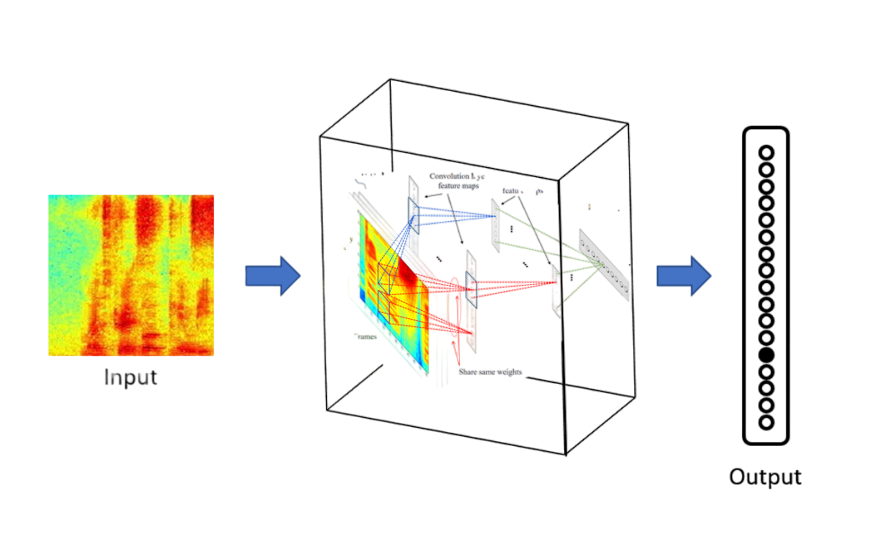
As with a number of my previous posts, I will be using a pretrained ResNet-18 model trained on the CUB2011 dataset; this will serve as the model under attack.
Scenario 1: Attacking a model with non-adversarial methods
This “attack” can also be seen as a model hardening test. I recommend running it on all computer vision models prior to deploying them. It tests the extent to which the model can handle common image transformations in the wild. Depending on the results, we might discover a cheap form of the evasion attack (applies to both black-box and white-box settings). The attack works as follows:
  1. Select a common image transform (e.g. rotation, brightness, contrast)
  2. Select a random test image
  3. Run the test image through the model and save the predicted class
  4. Run the transformed test image through the model and save the predicted class
  5. If #3 and #4 are different then increase counter
  6. Repeat steps 2-5 100 times to estimate the effect of the transform
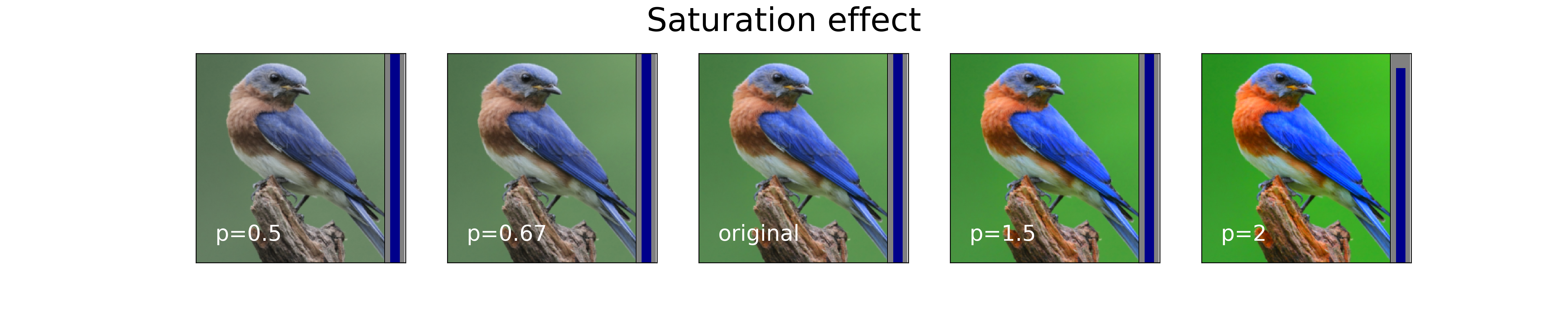
Results
The following plots visually demonstrate the effect of a single transform. The results (represented by the blue bar to the right of each image) represent the average performance of 100 test images. A higher bar signifies that the model is robust to that transform (i.e. the counter in step#5 was low).
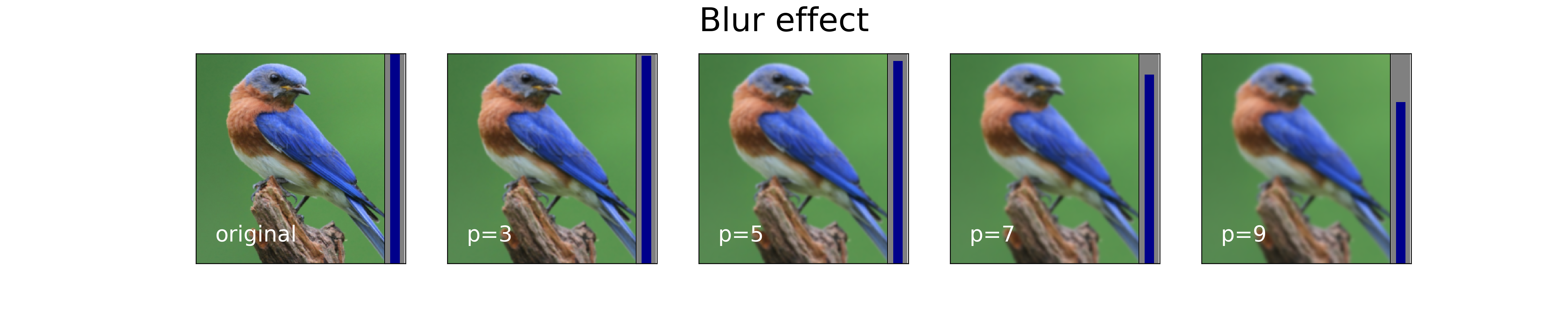
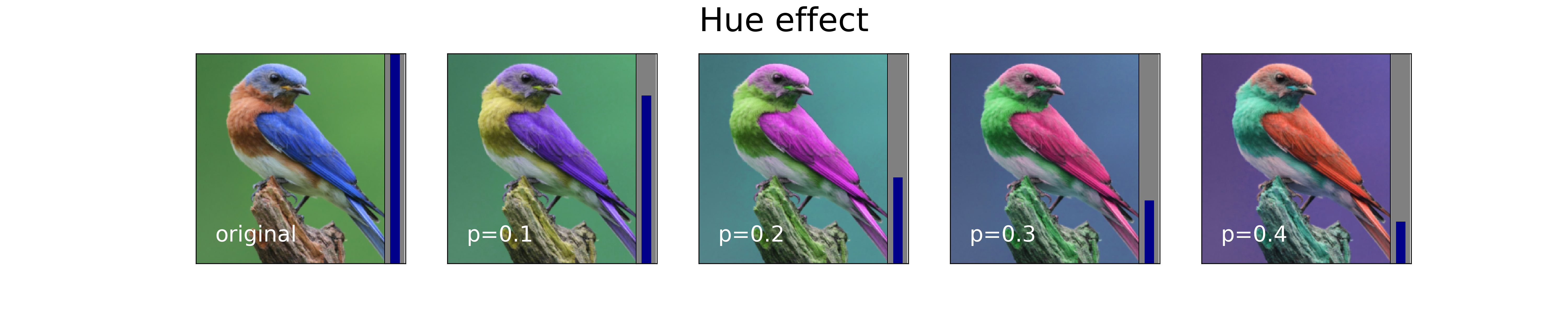
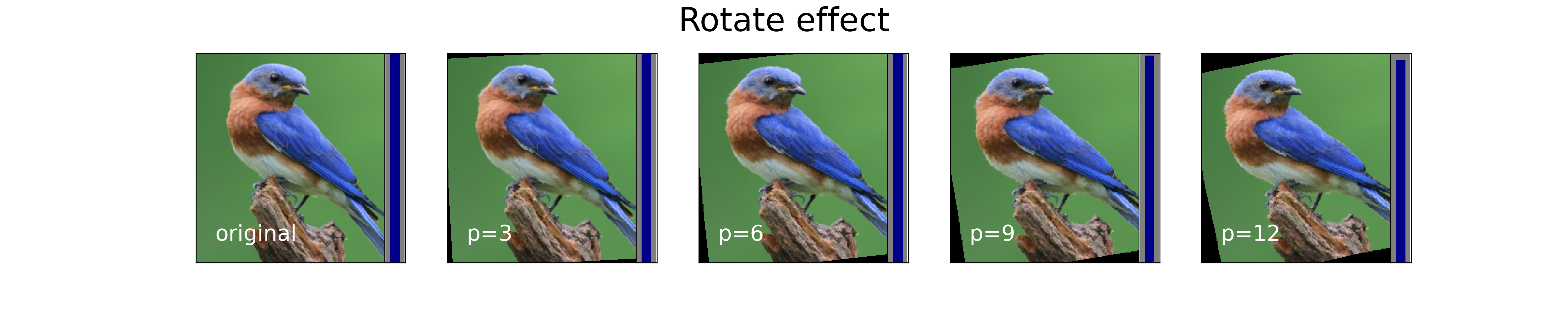
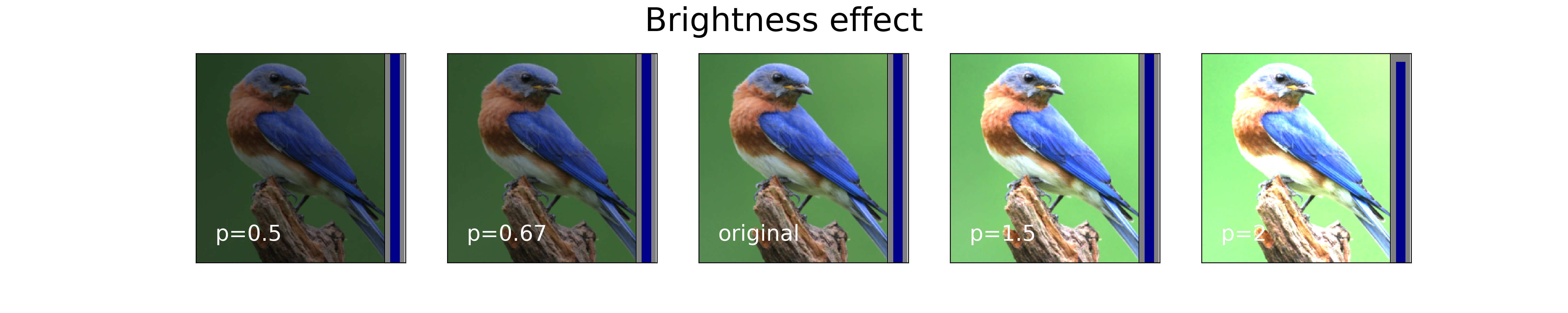
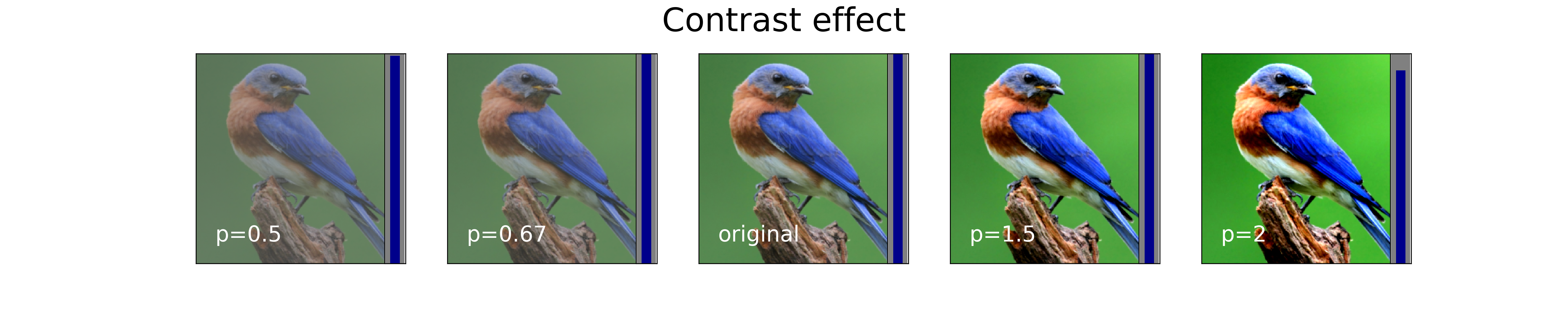
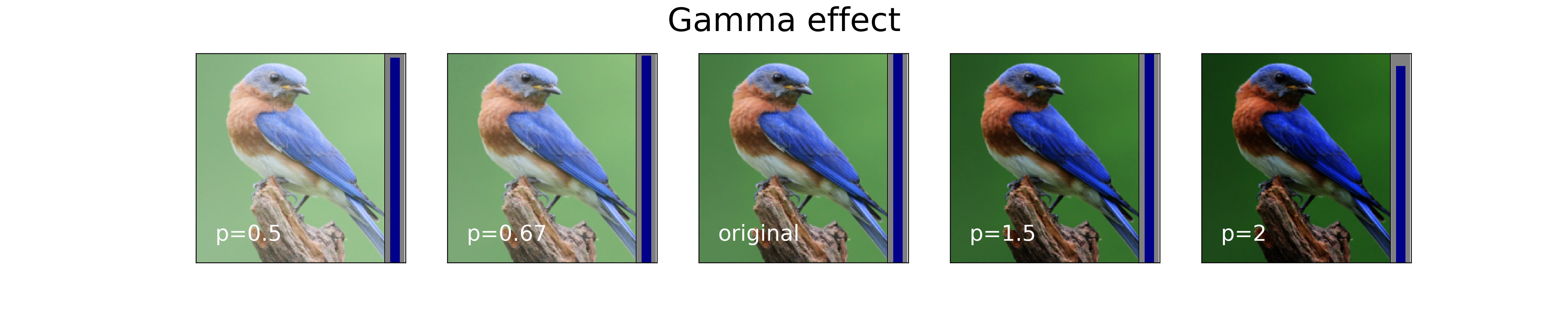
Discussion
The model under attack was relatively robust to subtle image transforms and should be expected to perform well in the wild. Hue was the only transform that significantly impacted performance and that is expected since color is a differentiating factor in bird species. Can we use hue as a cheap form of adversarial attack? No, because the hue transform would also fool a human. In other words, the hue transform fundamentally changes the input so it isn’t “fooling” anything. We next turn to more advanced methods.
Scenario 2: Attacking a model with adversarial methods
The goal of an evasion attack is to minimally modify an input (i.e. image) in such a way that the model alters its class prediction, but a human still percieves the original class. It’s this combination that makes the evasion attack so potent - humans don’t know anything is wrong and the machine is fooled. The attack succeeds because the altered image lies outside of the training distribution.
PGD
The Projected Gradient Descent (PGD) attack (Madry et. al, 2017) is an iterative optimization technique that seeks to find the most adversarial perturbation within a predefined constraint set. Here is psuedocode for the algorithm:
  1. Select an unmodified image as the target
  2. Select a random point within the allowed perturbation region of the target image
  3. Perform gradient descent on the model's loss function
  4. Project the perturbed input back into the feasible set after each iteration
This iterative process ensures that the adversarial perturbation remains within the defined constraints around the original input, making the adversarial example both effective and imperceptible to human observers.
However, the PGD attack has certain limitations that make it less practical for real-world applications:
- Over-optimization against one constraint
- Potential for unstable optimization
- Limited transferability to other models
Example
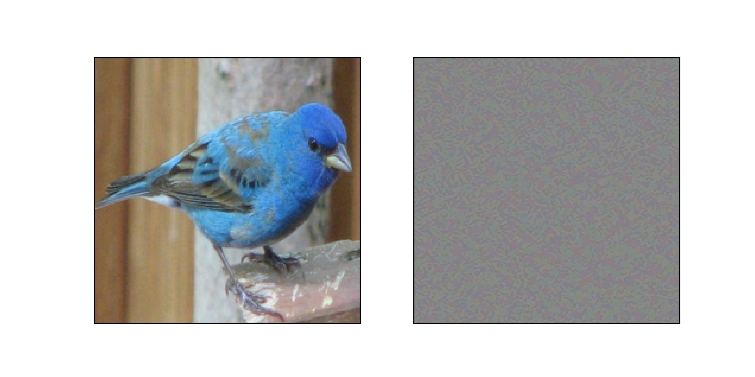
A successful example of a PGD attack (left). The modified image was classified differently than the original image, but the modifications are barely visible to the human eye. The modifications added to the original image are magnified 10x in the (right) image.
Carlini-Wagner
The Carlini & Wagner (C&W) attack is a powerful adversarial evasion attack that aims to generate adversarial examples that are misclassified by a target model. Adversarial examples are created by formulating an optimization problem, where the goal is to minimize the perturbation while ensuring the classifier mislabels the adversarial example. C&W is particularly notable for its ability to generate adversarial examples that are transferable across different models and defenses, making it a significant threat to the security of machine learning systems.
However, the C&W attack has certain limitations that make it less practical for real-world applications:
- Computational cost
- Requires domain-specific adaptations to shape the perturbations and the optimization problem depending on the type of data being manipulated
Example with L0 norm
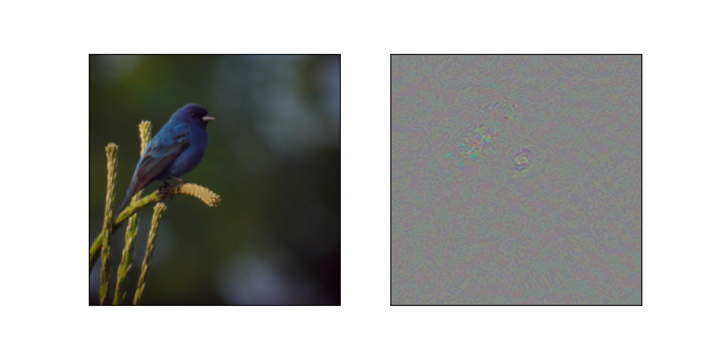
A successful example of a C&W attack (left). The modified image was classified differently than the original image. Although the modifications are mostly imperceptible, a small eye-like patch is visible in the magnitude-magnified image (right).
Example with LInf norm
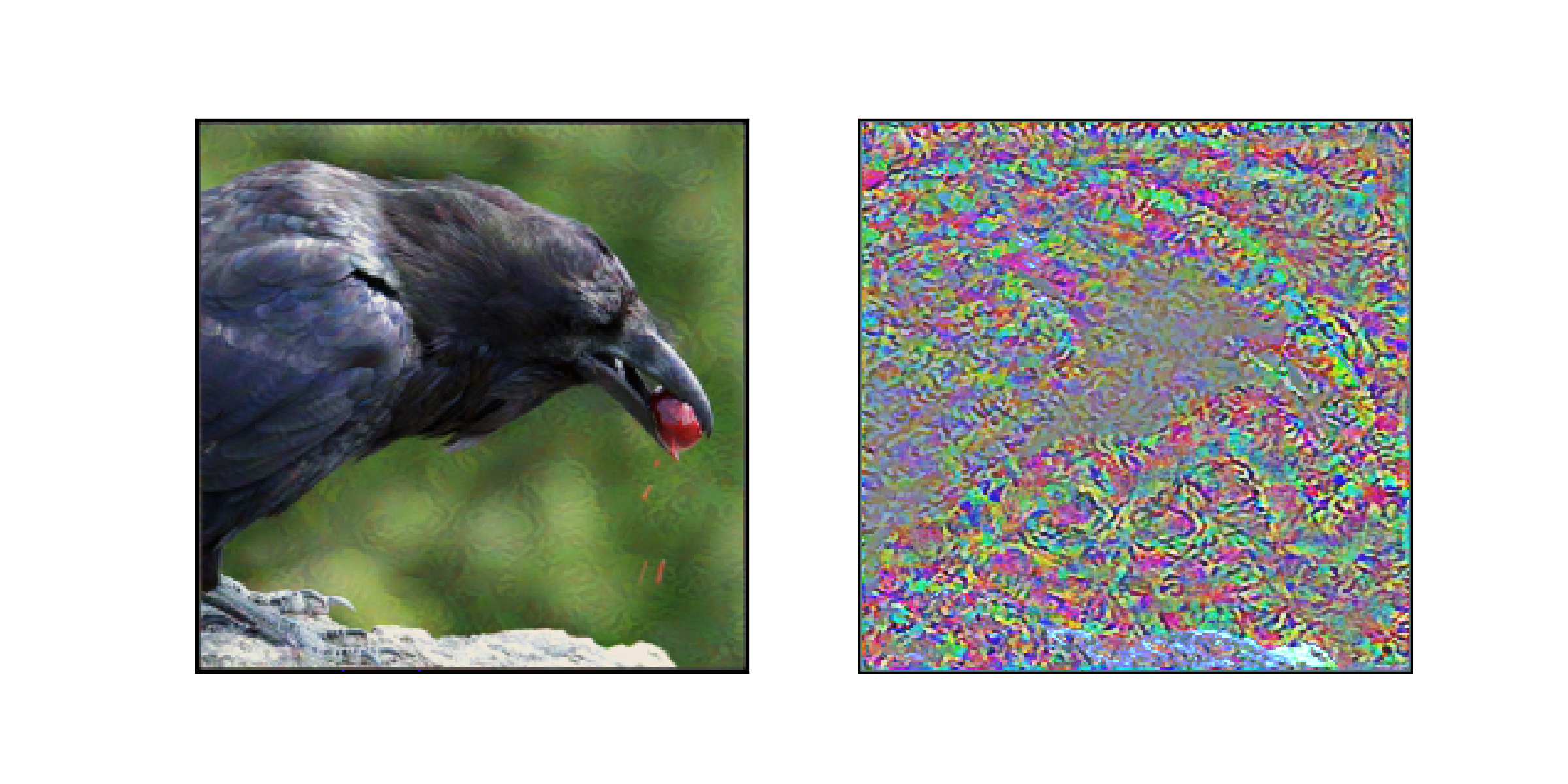
A successful example of a C&W attack (left). The modified image was classified differently than the original image. The modifications in this case are noticable and global in the original image and magnitude-magnified image (right).
Scenario 3: Defending a model with non-adversarial methods
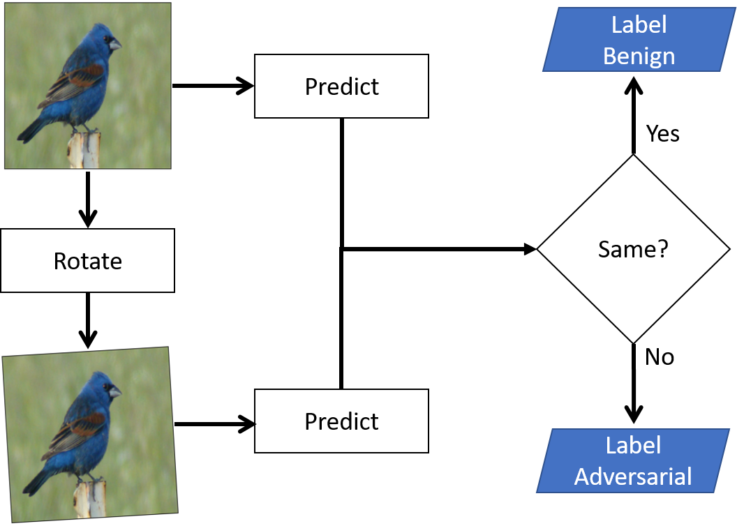
This scenario explores the exent to which non-adversarial methods can be used to defend a model from a strong adversarial attack (e.g. PGD or Carlini-Wagner). The defense exploits the fact that the evasion attack itself is typically brittle. In other words, the attack noise was calculated to minimize the amount of change in the input space to achieve the desired result. Therefore, it stands to reason that the attack may not be able to withstand additional transformations. We constrain the suite of transformations considered in Scenario #1 to only those transformations that maintained greater than 99% performance on natural images. This allows us to limit the amount of false positives in our adversarial detector to less than 1%.
Results
In the tables below we report the prediction rates for the best parameter combination per transformation type (e.g. rotation, brightness).
PGD
| Transformation | Parameter | Performance on natural images | Performance on adversarial images | Differential |
|---|---|---|---|---|
| rotate | 7 | 1 | 0.049505 | 0.950495 |
| brightness | 1.75 | 1 | 0.283019 | 0.716981 |
| saturation | 0.5 | 0.995305 | 0.441441 | 0.553864 |
| contrast | 1.5 | 1 | 0.454545 | 0.545455 |
| gamma | 1.5 | 1 | 0.555556 | 0.444444 |
| blur | 0 | 1 | 1 | 0 |
| hue | 0 | 1 | 1 | 0 |
CW-L0
| Transformation | Parameter | Performance on natural images | Performance on adversarial images | Differential |
|---|---|---|---|---|
| rotate | 7 | 1 | 0.114286 | 0.885714 |
| brightness | 1.6 | 1 | 0.558442 | 0.441558 |
| saturation | 0.5 | 0.995305 | 0.561905 | 0.4334 |
| gamma | 1.5 | 1 | 0.741935 | 0.258065 |
| contrast | 0.75 | 1 | 0.815126 | 0.184874 |
| blur | 0 | 1 | 1 | 0 |
| hue | 0 | 1 | 1 | 0 |
CW-LInf
| Transformation | Parameter | Performance on natural images | Performance on adversarial images | Differential |
|---|---|---|---|---|
| rotate | 7 | 1 | 0.819444 | 0.180556 |
| brightness | 1.75 | 1 | 0.910256 | 0.089744 |
| gamma | 1.5 | 1 | 0.939394 | 0.060606 |
| contrast | 1.5 | 1 | 0.943182 | 0.056818 |
| saturation | 1.5 | 1 | 0.944444 | 0.055556 |
| blur | 0 | 1 | 1 | 0 |
| hue | 0 | 1 | 1 | 0 |
Discussion
The highest average difference between performance on natural images and adversarial images is achieved by rotating images by 7 degrees. This transformation is ideal from a false-positive point of view as all natural images are unphased by it. NOTE: this does not mean that the predicted class is correct, only that the predicted class is not altered by rotating the image 7 degrees. Our ability to detect adversarial examples depends on the attack:
| TP rate | FP rate | |
|---|---|---|
| PGD | 0.95 | 0.0 |
| CW-L0 | 0.885 | 0.0 |
| CW-LInf | 0.18 | 0.0 |
The results are quite promising for PGD and CW-L0, but the CW-LInf attack proved to be more resilient (to all tested transformations). The results appear to confirm our hypothesis about the fragility of the evasion attacks - more subtle attacks are more easily detected precisely because they are more subtle. In other words, if the attack has a low signal-to-noise ratio then rotating the image has a better chance to render it ineffective.
Scenario 4: Defending a model with adversarial methods
Adversarial training is a technique used to enhance the robustness of machine learning models against adversarial examples. The simplest way to perform adversarial training is to include adversarial examples in the training set.
1. Train a model with the original training data
2. Use the model to generate adversarial examples
3. Add the adversarial examples (with correct labels) to the training data
4. Retrain the model
A more sophisticated approach called Robust training (Madry et. al, 2017) alters the optimization process itself in order to make models more resilient to adversarial perturbations. These perturbations are carefully crafted to deceive the model into making incorrect predictions.
Comparing detection and adversarial training
Adversarial training strengthens models intrinsically, while detection approaches focus on identifying adversarial examples during inference. Both play crucial roles in addressing the challenges posed by adversarial attacks.
- advantages of adversarial detection
- can defend against white-box and black-box threat models
- can be used to protect existing/pretrained models
- may work against UNKNOWN attacks
- advantages of adversarial training
- moderate success against all KNOWN attacks
NOTE: If you are training your own model then you can do BOTH!
Conclusion
This was a long post, so I will summarize the results here:
- It is good practice to test your model’s performance against non-adversarial image transformations.
- Evasion attacks (e.g. PGD and CW) can be used to alter the predictions of a model.
- Some evasion attacks (e.g. PGD and CW-L0) can be detected at inference time due to their lack of robustness against non-adversarial image transformations.
- Other evasion attacks (e.g. CW-LInf) may be rendered inneffective using adversarial training.
As ML adoption grows, understanding and addressing these vulnerabilities become crucial for maintaining system integrity and security. The code for this experiment can be found at my ML portfolio website.