Experiment 17

This post introduces Concept Bottleneck Models - an interpretable approach to machine learning.

Introduction to Explainable AI

Explainable machine learning models describe how and why a prediction was made. Experts in explainable AI (XAI) make a distinction between interpretabiliy and explainability: source

• Interpretability is the extraction of relevant sub-symbolic information from a machine-learning model concerning relationships either contained in data or learned by the model

• Explainability is the ability to translate this sub-symbolic information in a comprehensible manner through human-understandable language expressions

This blog post answers the following questions:

1. How do you make a machine learning model more interpretable and explainable?
2. What are the tradeoffs and when should you do it?

Experimental study

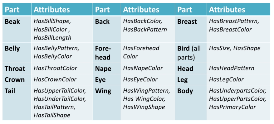
In order to demonstrate the benefits of XAI we will use a standard image classification task on well-known benchmark - CUB-200-2011, which contains 11,788 images of birds. This dataset is typically used for fine-grained classification since it contains over 200 species of birds. Additionally, for each image, it captures meta-data about each bird (i.e. 28 features including bill shape, wing shape, head color, etc.). This information will be critical to creating an interpretable model.

Image source

Establishing the baseline

Before we build an interpretable model, we will establish the performance of a non-interpretable model. For this dataset we will use a ResNet-18 pretrained model from the pytorchcv package.

from pytorchcv.model_provider import get_model 

cub_model = get_model('resnet18_cub', pretrained=True)

This model has 74.4% accuracy on the test set, which is impressive given that there are 200 classes and the classes are all similar because they are all birds. We will next describe how to adapt this model to be interpretable.

Concept Bottleneck Models

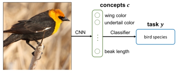
Deep learning models are powerful due to their ability to learn features that are discriminative to the prediction task. However, these features are not interpretable by humans, leading to the so-called “black box problem”. In an effort to make deep learning models more transparent, Concept Bottleneck Models (CBMs) make use of a human-interpretable feature layer called the “concept layer”. This layer contains features that are meaningful to a human and representative of the features necessary for a human to perform the same kind of prediction. The final prediction is made based on the values of the concept layer. There are two primary advantages of this approach:

1. Users can understand the feature values immediately before the prediction layer
2. Users can update the feature values to improve accuracy (sometimes called intervention)

image reference

Training a Concept Bottleneck Model

In the original paper the authors test three ways to train a Concept Bottleneck Model:

• Independent: learn a concept predictor (L_C) and learn a task predictor (L_Y)

• Sequential: learn a concept predictor (L_C) then learn a task predictor (L_Y | L_C)

• Joint: simultaneously learn concept predictor (L_C) and task predictor (L_Y | L_C)

The joint approach offered the best performance on the CUB dataset. However, because the concept and task predictors are trained simultaneously using a dual loss function is it prone to side-channel leaks, in which the task predictor drives the concept predictor to leak additional information about features that are not strictly related to the concepts. The extent to which this occurs affects the overall interpretability of the model.

Independent and sequential approaches offered similar performance on CUB and do not suffer from the side-channel leak problem. The independent approach is recommended for systems that anticipate high intervention rates because its task predictor is trained using ground truth concept values. The sequential approach is recommended when intervention is not likely and the concepts are difficult to predict. This allows the task predictor to learn to ignore concepts that may be difficult to predict.

Learning the concepts

There are 28 concepts in the CUB-200 dataset. These are expert-selected concepts relevant to the problem of bird species identification.

image reference

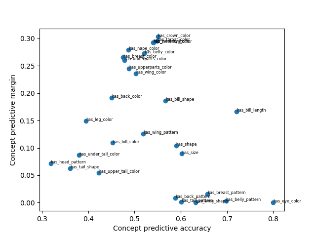
We will use the training data to learn to predict these features by creating one classifier per concept. The embedding features from the baseline ResNet-18 model serve as the input to each concept classifier. As you can see in the figure below, the ability to predict each concept varies greatly. This is partially due to the fact that the embedding space is optimized to differentiate at the class level (global prediction) rather than the individual concepts (local predictions).

Let’s take a closer look at a few examples:

• Head Pattern (33% accuracy) - this concept is difficult to predict from the embedded features; the classifier only performs marginally better than the base rate (+7% better)
• Eye Color (80% accuracy) - this concept is the most accurately predicted concept; but it does not perform better than the base rate, suggesting that this feature is not informative and predicts that birds have black eyes regardless of input
• Crown color (55% accuracy) - although this concept is not among the most accurately predicted, it does perform significantly higher than the base rate (+30% better) suggesting that the embedded features at least partially capture this information

Learning the classes

Because the performance of the concept predictors was relatively low, we will use a sequential training approach. After learning one concept predictor per concept L_Ci, we use the predicted concepts (rather than the ground truth concepts) to learn the task predictor.

Results

	Backbone	Interpretable features	Concept labels required	Accuracy
CBM	ResNet-18	Y	Y	0.594
Baseline	ResNet-18	N	N/A	0.744

We added interpretability to our model at the cost of about 25 points of accuracy. This would be an unacceptable tradeoff for most real-world applications. Even though the overall accuracy is low, if either the accuracy of the concept predictor or task predictor is independently high then they can still be useful in certain contexts.

• Expert assistant: This scenario assumes the system is being used by a highly trained user (e.g. ornithologist for CUB). The concept predictor (with high accuracy) can save the expert time by pre-populating values for the concept features. The expert then performs a final review of the concept features and assigns the final class label (e.g. species of bird for CUB).
• Psuedo-expert: This scenario assumes the system is being used by non-skilled users (e.g. Mechanical Turk workers). The worker is able to make simple observations about the image (e.g. what is the color of the bird’s wing, which of the following shapes most closely matches the bird’s beak, etc.). The task predictor (with high accuracy) then assigns the species of bird given the observations.

Discussion

Limitations of CBMs

We have already observed the first limitation of Concept Bottleneck Models - they don’t tend to be as accurate as non-interpretable models for real-world applications. This gap can be reduced using a residual modeling technique such as the one proposed in Yuksekgonul, Wang, & Zou, (2022), which splits the model’s predictions into an interpretable part and a non-interpretable part.

Another limitation is the assumption of the concept labels themselves. The data labeling cost for such a dataset is significantly higher than one that only collects the task labels. Furthermore, the concepts themselves are difficult to get right without expert input. One solution, proposed in Oikarinen et. al (2023), uses a combination of a large language model (GPT-3) and a multimodal foundation model (CLIP) to extract concepts for any task. See paper for details. The reported accuracy of their approach is included in the table below.

Limitations of ResNet-18 backbone

I have made it tradition to incorporate DINOv2 into my ml-portfolio series posts. In this post, I replaced the ResNet-18 backbone with DINOv2 and the accuracy improves 15 points. I can’t think of many applications that would prefer an interpretable model with 60% accuracy over a non-interpretable model with 90% accuracy. NOTE: Although the DINOv2 features were better for overall task accuracy, they did not significantly improve concept accuracy.

	Backbone	Interpretable features	Concept labels required	Accuracy
CBM	ResNet-18	Y	Y	0.594
Label-free CBM	ResNet-18	*Y	N	0.743
Baseline	ResNet-18	N	N/A	0.744
Baseline	DINOv2	N	N/A	0.905

*Features in this space take on continuous values correlated with human relatable concepts.

Alternative approaches to interpretability

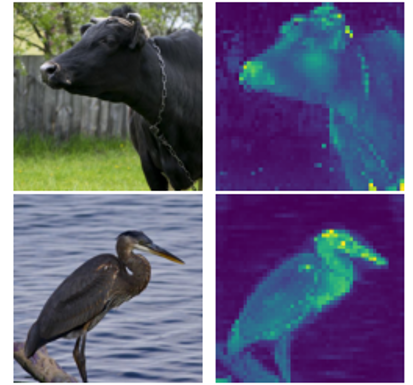
Saliency/attention maps are a common post-hoc interpretability technique that can be applied to any deep learning model. The purpose of these maps is to show the user which input features the model used for to perform most of their computations (i.e. paid the most attention to). They have one advantage over Concept Bottleneck Models in that they do not affect accuracy.

image reference

But for the purposes of interpretability, I find that the approach falls short. At best it confirms for the user that the expected parts of the input were used to make a decision and not a spurious object (i.e. a common example is that the class “frisbee” is assigned to images containing large amounts of green grass). But attention maps fail to explain anything about the internal features of the model and its decision process. DINOv2 attention maps tend to highlight a single, main subject in an image. But it doesn’t do that because it knows the difference between a cow and a blue heron; it was trained in a totally unsupervised way! Furthermore, attention maps do not provide a mechanism for intervention.

Conclusion

In this post I demonstrated how to make a machine learning model more interpretable and explainable. I also discussed the tradeoffs and alternative uses for such models when their accuracies do not perform at practical levels. The code for this experiment can be found at my ML portfolio website.