Experiment 10
Introducing the Quantum Smalltalk series
In this series I am going to introduce you to some of my favorite quantum experiments while modeling those experiments in Pharo Smalltalk. We will explore the quantum properties of superposition and entanglement. Our experimental model is rather simple - the optical devices typically used in such experiments (i.e. beam splitters, polarizers, mirrors) will be modeled using complex-valued linear transformations. Although the results of matrix multiplication may not surprise you, I hope that the results of these experiments will. I could have called this the “Complex-valued matrix multiplication with Smalltalk series,” but that doesn’t have quite the same ring.
Why Smalltalk?
I chose Smalltalk for this series because it allows me to quickly implement an internal (or embedded) domain specific language (DSL) to describe the quantum experiments. You will become more familiar with the DSL as we progress, but here is a sample:
Photon new
	beamSplitter;
	blockLowerPath;
	mirror;
	beamSplitter;
	detector.
A good DSL simplifies the code to allow you to focus on the concepts rather than the syntax. A great DSL is self-explanatory, allowing a domain expert (in this case a physicist) to use it without any previous programming experience. I don’t know any physicists so this is at least a good DSL.
The Mach-Zehnder setup
All of the experiments in this series will be variations of the Mach-Zehnder interferometer. It was originally proposed in 1891 to measure phase shifts between the two paths caused by a sample, but it has since been adapted to study a variety of quantum effects. Why aren’t we using the double-slit experiment? It may be the most iconic quantum experiment, but it is also difficult to model because it requires differential equations. We can demonstrate multiple quantum properties (i.e. superposition and entanglement) using the much simpler Mach-Zehnder setup.
Feynman once claimed that any question in quantum mechanics could be answered using the double-slit experiment. (But of course he said it as only he could, “You remember the experiment with the two holes? It’s the same thing.”)
The purpose of the first experiment is to familiarize yourself with the:
- experimental setup and optical components used
- modeling approach (i.e. matrix multiplication)
- Smalltalk DSL describing the experimental setup
Basic optical components
This section describes the optical components used in the first 2 experiments. Each component is described in common language as well as its equivalent mathematical transformation. Credit: All of the diagrams and mathematical notation used in this series follows from MIT’s Quantum Physics 1; this is an excellent course taught by Dr. Barton Zwiebach.
Photon Emitter
Luckily for us, all of the components have rather descriptive names. In this experiment, we will not be using a coherent laser as the source, but instead a single photon will traverse the optical path (or paths) of the experiment. When a photon is emitted on the upper beam it is represented by the following probability amplitudes:
Beamsplitter
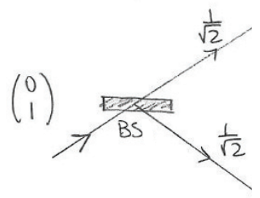
If you shine a laser at a balanced beam splitter (the only kind we model here) then exactly 50% of the light is transmitted and the remaining 50% is reflected (also undergoing a phase shift of PI). What happens if you send a single photon instead of a laser? Hopefully you will be able to answer that after the second experiment, but for now assume that there is a 50% chance that it gets reflected and a 50% chance that it gets transmitted. This is represented mathematically by:
An aside on probabilities
The careful reader will notice that the result of a photon passing through a beamsplitter yields 1/sqrt(2) instead of 1/2. That is because this number represents a probability amplitude.
You can convert a probability amplitude to a probability by taking its magnitude and squaring it.
Mirror
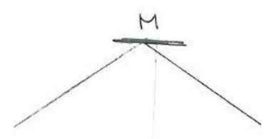
A mirror reflects an incoming photon while undergoing a phase shift of pi.
Block
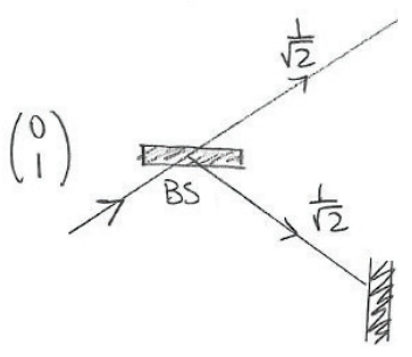
A block absorbs an incoming photon, preventing it from reaching any downstream components. In the diagram above, the beamsplitter produces a 50% chance that the photon is absorbed by the block and a 50% chance that the photon is allowed to continue on the upper path.
Photon Detector
This component detects a single photon. Most of the experimental setups used in this series will involve 2 detectors: D0 measuring the upper path and D1 measuring the lower path. Just as the emitter emits a real photon, the detector detects a real photon (i.e. it does not measure probability amplitudes or probabilities). The mathematical equivalent of the photon detector would be to sample the probabilities of all possible end-states of the photon (they should add up to 1). We will forgo this step and instead just report the associated probabilities.
Experiment #10
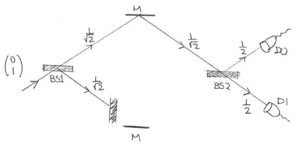
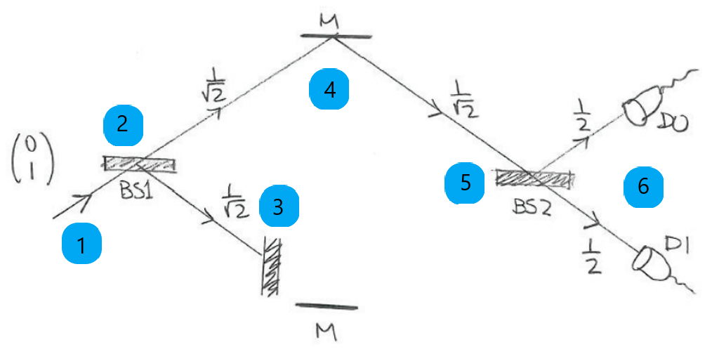
This experiment is relatively straightforward - its result is intuitive and agrees with a more classical interpretation. The setup includes:
- 1 photon emitter
- 1 block
- 2 beam-splitters
- 2 mirrors
- 2 detectors
Before we do the math, let’s guess what might happen if we run this experiment 100 times. If the beamsplitters act like a random coin (heads the photon transmits, tails it reflects) then one might expect the following outcome:
| Photon outcome | counts |
|---|---|
| Detected at D0 | 25 |
| Detected at D1 | 25 |
| Absorbed by block | 50 |
Next let’s run the experiment and see if the calculated probabilities agree with our intuition (I’ll defer the Smalltalk code for now and just show the output report).
Emitting a photon from lower path. >> #(0 1)
Photon passing through a beam splitter. >> #(0.4999999999999999 0.4999999999999999)
Photon's path blocked on lower path. >> #(0.4999999999999999 0)
Photon bouncing off of a mirror. >> #(0.0 0.4999999999999999)
Photon passing through a beam splitter. >> #(0.2499999999999999 0.2499999999999999)
Photon finally detected with following probabilities: >> #(0.2499999999999999 0.2499999999999999)
| Photon outcome | probability |
|---|---|
| Detected at D0 | 0.25 |
| Detected at D1 | 0.25 |
| Absorbed by block | 0.50 |
The computed probabilities agree with our intuition!
Summary
Experiment 10 laid the groundwork for the quantum properties we want to explore in the rest of the series. It introduced the optical components and how they are modeled mathematically. However, I have not yet shown the Smalltalk code because it is not as important as the rest. If you want to better understand how to compute the probability amplitudes at an arbitrary point in the path then I would encourage you to consider watching the first few lectures of MIT’s Quantum Physics 1.
Appendix: The Smalltalk code
I was surprised at how simple the Smalltalk DSL code turned out to be. It’s almost anti-climactic at this point, but the code almost line-by-line describes the order of the components in the experiment. Please keep in mind that the mathematical complexity lies beneath this layer and is hidden from the user. The full Pharo package can be found at dlfeps/MZI.
1 Photon new
2   beamSplitter;
3   blockLowerPath;
4   mirror;
5   beamSplitter;
6   detector.
